


Polynomial Functions and Their Graphs
Math 1310
Section 4.1: Polynomial Functions and Their Graphs
A polynomial function is a function of the form

where  are real numbers
and n is a whole number.
are real numbers
and n is a whole number.
The degree of the polynomial function is n. We call the
term  the leading term, and
 is called the leading coefficient.

Our objectives in working with polynomial functions will be, first, to gather
information
about the graph of the function and, second, to use that information to generate
a reasonably good
graph without plotting a lot of points. In later examples, we’ll use information
given to us about
the graph of a function to write its equation.
Graph Properties of Polynomial Functions
Let P be any nth degree polynomial function with real coefficients. The graph of
P has the
following properties.
1. P is continuous for all real numbers, so there are no breaks, holes, jumps in
the graph.
2. The graph of P is a smooth curve with rounded corners and no sharp corners.
3. The graph of P has at most n x-intercepts.
4. The graph of P has at most n – 1 turning points.
Example 1: Given the following polynomial functions, state the leading term, the
degree of the
polynomial and the leading coefficient.


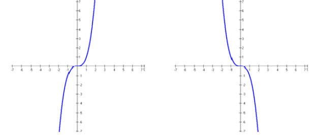
We’ll start with the shapes of the graphs of functions of
the form 
You should be familiar with the graphs of  and
and 
The graph of  is even, will resemble the
graph of , and the graph
is even, will resemble the
graph of , and the graph
of  n is odd, will resemble the graph of


Next, you will need to be able to describe the end
behavior of a function.
End Behavior of Polynomial Functions
The behavior of a graph of a function to the far left or far right is called its
end behavior.
The end behavior of a polynomial function is revealed by the leading term of the
polynomial
function.
1. Even-degree polynomials look like . 

2. Odd-degree polynomials look like.
Next, you should be able to find the x intercept(s) and
the y intercept of a polynomial function.
Zeros of Polynomial Functions
You will need to set the function equal to zero and then use the Zero Product
Property to find the
x-intercept(s). That means if ab = 0, then either a = 0 or b = 0 . To find the y
intercept of a function,
you will find f (0).
Example 2: Find the zeros of:


In some problems, one or more of the factors will appear
more than once when the function is
factored. The power of a factor is called its multiplicity. So given
 then
then
the multiplicity of the first factor is 3, the multiplicity of the second factor
is and the multiplicity of
the third factor is 1.
Description of the Behavior at Each x-intercept
1. Even Multiplicity: The graph touches the x-axis, but does not cross it. It
looks like a parabola
there.
2. Multiplicity of 1: The graph crosses the x-axis. It looks like a line there.
3. Odd Multiplicity greater than or equal 3: The graph crosses the x-axis. It
looks like a cubic there.
You can use all of this information to generate the graph
of a polynomial function.
• degree of the function
• end behavior of the function
• x and y intercepts (and multiplicities)
• behavior of the function through each of the x intercepts (zeros) of the
function
Steps to graphing other polynomials:
1. Determine the leading term. Is the degree even or odd? Is the sign of
the leading coefficient
positive or negative?
2. Determine the end behavior. Which one of the 4 cases will it look like
on the ends?
3. Factor the polynomial.
4. Make a table listing the factors, x intercepts, multiplicity, and describe
the behavior at each x
intercept.
5. Find the y- intercept.
6. Draw the graph, being careful to make a nice smooth curve with no sharp
corners.
Note: without calculus or plotting lots of points, we don’t have enough
information to know how high
or how low the turning points are
Example 3: Find the x and y intercepts. State the degree of the function.
Sketch the graph of


Example 4: Find the x and y intercepts. State the
degree of the function. Sketch the graph of


Example 5: Find the x and y intercepts. State the
degree of the function. Sketch the graph of

Example 6: Find the x and y intercepts. State the
degree of the function. Sketch the graph of

Example 7: Write the equation of the cubic
polynomial P(x) that satisfies the following conditions:
zeros at x = 3, x = -1, and x = 4 and passes through the point (-3, 7)
Example 8: Write the equation of the quartic
function with y intercept 4 which is tangent to the x
axis at the points (-1, 0) and (1, 0).
Math 1310
Section 4.2: Dividing Polynomials
In this section, you’ll learn two methods for dividing polynomials, long
division and synthetic
division. You’ll also learn two theorems that will allow you to interpret
results when you divide.
Suppose P(x) and D(x) are polynomial functions and D(x) ¹ 0. Then there are
unique polynomials
Q(x) (called the quotient) and R(x) (called the remainder) such that P(x) = D(x)
*Q(x) + R(x) .
We call D(x) the divisor. The remainder function, R(x) , is either 0 or of
degree less than the degree
of the divisor.
You can find the quotient and remainder using long division. Recall the steps
you
learned in elementary school to perform long division:
Example 1: Divide

Example 2: Divide

Example 3: If  and
and
 , in
, in  .
.
Often it will be more convenient to use synthetic division
to divide polynomials. This method is
easy to use, as long as your divisor is x ± c , for any real number c.
Dividing Polynomials Using Synthetic Division
Example 4: Divide using synthetic division

Example 5: Divide using synthetic division

Example 6: Divide using synthetic division

Here are two theorems that can be helpful when working
with polynomials:
The Remainder Theorem: If P(x) is divided by x - c, then the remainder is
P(c) .
The Factor Theorem: c is a zero of P(x) if and only if x - c is a factor
of P(x), that is if the
remainder when dividing by x - c is zero.
You can use synthetic division and the remainder theorem to evaluate a function
at a given value.
Example 7: Use synthetic division and the remainder theorem to find P(3)
for

Example 8: Determine if x + 2 is a factor of

And you may also need to work backwards.
Example 9: Find a polynomial with a degree of 4 with zeros at -3, 0, 2,
5.
Example 10: Find a polynomial of degree 3 with zeros at 0, 2 and -3.
Math 1310
Section 4.3: Roots of Polynomial Functions
You’ll need to be able to find all of the zeros of a polynomial. You’ll now be
expected to find both
real and complex zeros of a function.
A polynomial of degree n ³ 1has exactly n zeros, counting all multiplicities.
To find all zeros, you’ll factor completely. From the factored form of your
polynomial, you’ll be
able to read off all the zeros of the function.
If c is a zero of a polynomial P, then x = c is a root of the equation P(x) = 0.
If your polynomial has real coefficients, then the polynomial may have complex
roots. Complex
roots occur in pairs, called complex conjugate pairs. This means that if a + bi
is a root of P then so
is a - b.
Note: 
Example 1: Find the zeros of the polynomial write the polynomial in factored
form and then state
the multiplicity of each zero. (Sometimes it may be easier to factor the
polynomial first, then find
the zeros.)


You can also work backwards to writing a polynomial with
integer coefficients that meets stated
conditions.
Example 2: Find a 3rd degree polynomial with integer coefficients given -5, and
i are zeros
Example 3: Find a polynomial with integer coefficients given the zeros at 2 and 2 - 5i.
Example 4: Write a polynomial with integer coefficients
with degree 4 and zeros at -3
(multiplicity 2) and - 3i .
Example 5: Write a polynomial with integer coefficients with degree 3 and zeros
at 5 and 4 + i
with a constant coefficient of 170.